Mini Autonomously Navigating Robot

Github

---

Overview

The goal of this project is to navigate a course autonomously using Aruco markers for localization and an Extended Kalman Filter (EKF) for accurate state estimation. The robot platform used is a Moorebot Scout which is a small, omni-directional robot equipped with a wide angle camera and compute that supports ROS.

---

System Architecture

The system consists of 4 main components:

1. Perception: The robot uses the camera to detect Aruco markers placed on the course. The camera captures images and processes them to identify the markers and their positions.
2. Localization: The robot uses the detected markers to estimate its position and orientation on the course. This is done using an Extended Kalman Filter (EKF) which fuses the camera measurements with the robot's odometry data to provide a more accurate state estimate.
3. Planning: The robot uses a PD controller to determine velocity commands based on the estimated position and the distance to the next waypoint.
4. Control: The robot executes the commands generated by the planning module to move towards the next waypoint. Then the process repeats.

---

Perception

For the robot to percieve it's location we used Aruco markers as landmarks. Aruco markers are a type of fiducial marker that can be easily detected by computer vision algorithms. As the markers have a known size, shape and pattern, they can be used to determine the position and orientation of the robot in 3D space. The markers are placed on the course at known locations and are detected by the robot's camera.

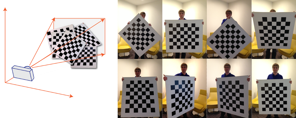
Before any markers can be detected, the camera must be calibrated to correct for lens distortion. By taking multiple images of a chessboard pattern from different angles and distances, the camera's intrinsic and extrinsic parameters can be found and used to undistort the images. For this project I used the Matlab Image Processing Toolbox.

The detection is achieved using OpenCV's aruco module which provides functions for detecting and estimating the pose of the markers. Below is the code that returns the marker IDs, positions and rotation vectors of the detected markers in the image.

# markers.py

import cv2 as cv
import numpy as np
import cv2.aruco as aruco

def detect_markers(image):
    """
    Detects ArUco markers in the given image and returns their pose.

    Returns:
        markerIds (np.ndarray): Detected marker IDs.
        marker_position (np.ndarray): Translation vector (x, y, z) of the first detected marker.
        marker_rotation (np.ndarray): 3x3 rotation matrix of the first detected marker.
    """
    # Load predefined ArUco marker dictionary and detection parameters
    dictionary = aruco.getPredefinedDictionary(aruco.DICT_6X6_250)
    parameters = aruco.DetectorParameters()
    detector = aruco.ArucoDetector(dictionary, parameters)

    # Detect markers in the image
    marker_corners, marker_ids, _ = detector.detectMarkers(image)

    # Camera calibration parameters from previous calibration
    camera_matrix = np.array([
        [675.9452775628, 0, 529.8337503423],
        [0, 682.3705999404, 307.1502458470],
        [0, 0, 1]
    ])
    dist_coeffs = np.array([-0.4149188226, 0.1203670324, 0.0, 0.0, 0.0])

    marker_position = None
    marker_rotation = None

    if marker_ids is not None:
        # Draw detected markers on the image
        aruco.drawDetectedMarkers(image, marker_corners, marker_ids)

        # Estimate pose of each detected marker
        for i in range(len(marker_ids)):
            rvec, tvec, _ = aruco.estimatePoseSingleMarkers(
                marker_corners[i], 0.05, camera_matrix, dist_coeffs
            )
            rvec = rvec[0]
            tvec = tvec[0] # Translation vector, x is right, z is forward

            # Convert rotation vector to rotation matrix
            R, _ = cv.Rodrigues(rvec)

            # Store pose of the first marker only
            marker_position = tvec.reshape(3,)
            marker_rotation = R
            break

    else:
        print("No markers detected.")
        return None, None, None

    return marker_ids, marker_position, marker_rotation

Now that we have the marker positions from the perspective of the robot, we can use them to get the position of the robot with respect to the world frame.

Using the transforms above, we get a measurement of the robot's state. This state is represented as a vector (x, y, θ).

---

Localization

The next step is to determine the robot’s position (x, y, θ) on the map, which is known as localization. In this project we have two sources of information to determine the robot's position: the commands we give to the robot (forward velocity and angular velocity) and the measurements we get from the ArUco markers. However, both of these sources of information are noisy and can be unreliable. This is where the Extended Kalman Filter (EKF) comes in. By fusing both the command inputs and the measurements from the ArUco markers, we can get a more accurate estimate of the robot's position than if we relied on either source alone.

To do this, the EKF will keep track of two key parameters:

1. State estimate x – in this case the robot's current position and orientation (x, y, θ)
2. Covariance matrix P – represents the uncertainty in the state estimate

As the robot moves and receives new measurements, the EKF updates its state estimate and covariance matrix. If tuned correctly, the uncertainty in the state estimate will decrease over time, causing the EKF to converge to the true state of the system.

The EKF operates in two main steps: Propagation (Prediction) and Update (Correction).

EKF: Propagation Step

In the propagation step, the system predicts its future state based on its current state and a motion model. In this project, the motion model is a differential drive model, which takes the inputs of the forward velocity v and the angular velocity ω to predict the next state of the robot.

Using the previous state (Xk), control input (uk), and assuming no process noise (represented by the zero vector), the EKF predicts the next state (Xk+1).

Plugging in the differential drive model, this can be expressed as:

Next, we need to determine the new covariance matrix P, which represents the uncertainty in the current state. As we predict further into the future, our estimates naturally become more uncertain. The matrix math below will take care of this.

Where 'A' is the jacobian of the differential drive model (the model must be linearised). Pk is the previous covariance. And Q is the process noise matrix, a tuning parameter, representing any error that could be in the model such as external disturbances.

EKF: Update Step

In the update step, the EKF refines its predicted state by incorporating new sensor measurements. In this case, position observations from ArUco markers. This step adjusts both the state estimate x and the uncertainty P using the incoming measurement z.

The update consists of three main parts: calculating the Kalman Gain, updating the state, and updating the covariance matrix.

1. Calculate the Kalman Gain

The Kalman Gain K determines how much the filter should trust the new measurement relative to the prediction. It is computed using the following equation:

Where:

• P is the predicted state covariance
• H maps the state space to the measurement space
• R is the measurement noise covariance matrix

The Kalman Gain acts as a weighting factor. A high K (close to 1) means the measurement is trusted more, while a low K (close to 0) means the prediction is trusted more.

2. Update the State Estimate

Next, the filter updates the predicted state using the new measurement. In this case we assume the measurement from the ArUco Markers gives direct observations of the robot's position and orientation:

We update the state estimate using the measurement z and the predicted measurement Hx. In this case Hx is simply the current state estimate. The Kalman Gain acts to adjusts the predicted state based on how different the actual measurement z is from the expected one Hx.

3. Covariance Update

Finally, the covariance matrix is updated to reflect the reduced uncertainty after incorporating the measurement:

Where I is the identity matrix.

These updates help the EKF continuously refine the robot's estimate of its position and orientation with each new measurement.

EKF: Tuning

The performance of the EKF depends heavily on how it is tuned. Proper tuning determines how the filter balances trust between the motion model and the sensor measurements. This is controlled primarily through three matrices: the initial covariance matrix P, the process noise matrix Q, and the measurement noise matrix R.

Initial Covariance Matrix P

The initial covariance matrix P represents the uncertainty in the initial estimate of the robot’s position and orientation. Adjusting this matrix is beneficial at the beginning of the system, as the robot’s state is unknown. However, as the filter progresses, the values of the initial P matrix don’t significantly matter, as they are corrected by the algorithm. Here are the tuning values for the robot:

self.P = np.array([[0.1, 0, 0],
                   [0, 0.1, 0],
                   [0, 0, 1]])

• The diagonal values represent how confident we are in each state variable initially (x,y,θ).
• The high value of 1 for θ (orientation) implies that the filter starts with more uncertainty in the robot’s heading than in its x or y position. This is because I placed the robot at the start location with varying orientations.

Process Noise Matrix Q

This matrix models uncertainty in the motion model such as wheel slippage or imperfect control inputs. It is a tuning parameter that defines how much error we expect in the robot’s motion. Here are the tuning values for the robot:

SIGMA_V = 0.1
SIGMA_W = 0.1

self.Q = np.array([[SIGMA_V**2, 0, 0],
                   [0, SIGMA_V**2, 0],
                   [0, 0, SIGMA_W**2]])

• SIGMA_V and SIGMA_W represent standard deviations for the forward (v) and angular (ω) velocity commands.
• Larger values in Q mean you trust your motion model less, which causes the EKF to rely more on measurements for updates.

Measurement Noise Matrix R

This matrix models the uncertainty in the sensor measurements, specifically the readings from ArUco markers. Tuning this matrix made the biggest difference in performace. Here are the tuning values for the robot:

MEAS_NOISE = 1.5

self.R = np.array([[MEAS_NOISE**2, 0, 0],
                   [0, MEAS_NOISE**2, 0],
                   [0, 0, MEAS_NOISE**2]])

• A larger R value instructs the EKF to reduce its reliance on measurements, leading to smoother, slower updates that are less reactive to sensor noise. During testing, increasing this value resulted in the robot’s estimate becoming smoother and less prone to sudden fluctuations. However, excessively increasing this value would make the robot sluggish in responding to markers and failing to correct its position. As a result, it became too slow to be responsive.

Overall, proper tuning ensures that the EKF converges quickly and remains stable, providing accurate localization even in the presence of noise.

For more information on Kalman Filtering checkout this video series by iLectureOnline.

---

Planner

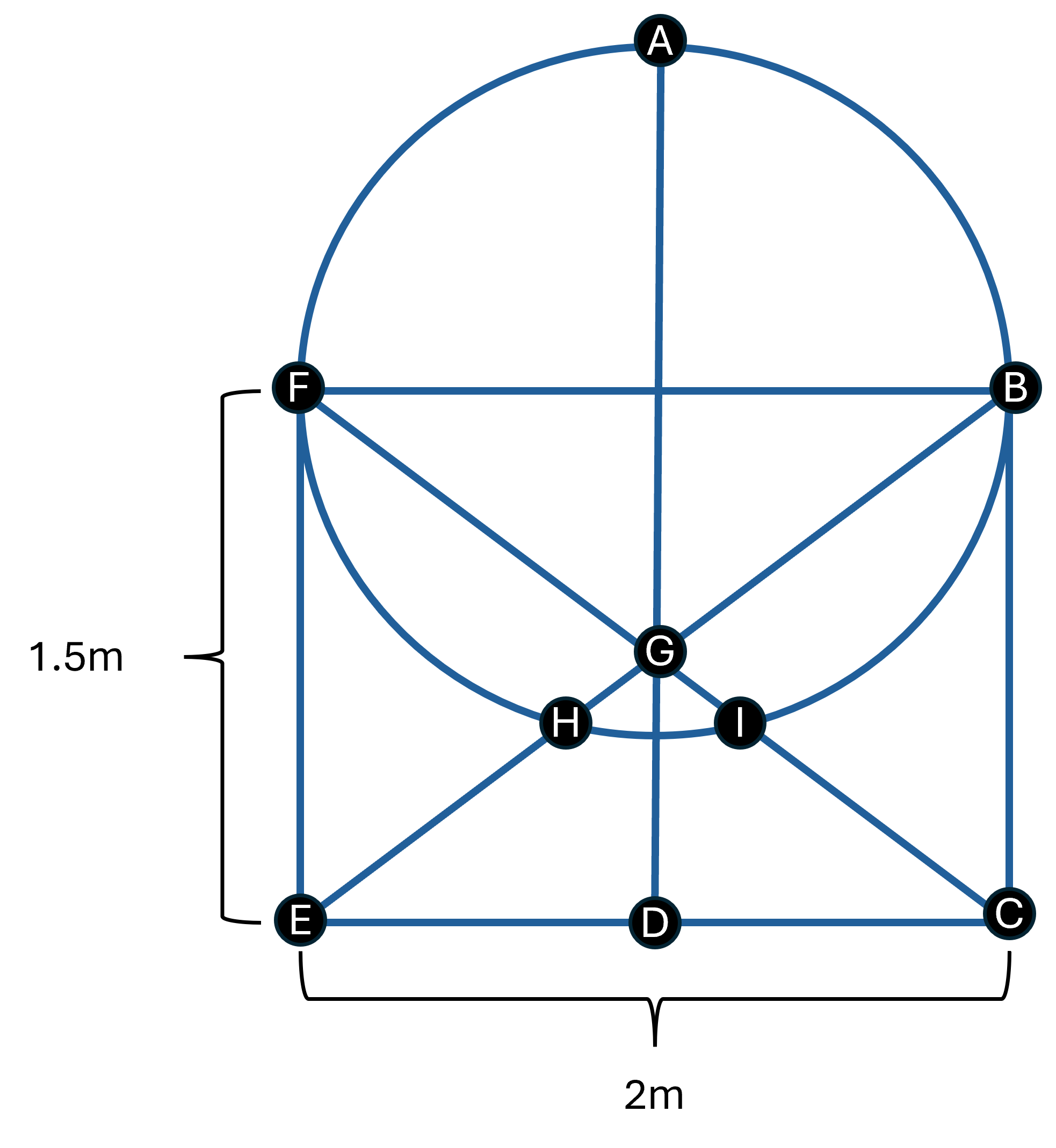
Now that we have the robot’s location, we need to determine how to command the robot to it's destination. The goal of this project is to navigate the outer perimeter of the course (EFABCDE, as shown below).

The planner is divided into two parts: the global planner and the local planner.

Global Planner

The global planner’s primary function is to determine the overall path that the robot should follow. This path is pre-determined based on our goal (EFABCDE). The path is represented as a list of waypoints that the robot should follow. These waypoints are defined in the world frame and serve as the robot’s reference points. Once the robot reaches within a specified distance of a waypoint, it transitions to the next waypoint and continues until it reaches the end of the path.

Local Planner

The local planner’s responsibility is to determine how to follow the determined path. The local planner utilizes a PD controller to calculate the velocity commands necessary to reach the next waypoint. The PD controller takes the current position of the robot and the position of the next waypoint as input and computes the error in both the x and y directions. This error is then used to determine the velocity commands for the robot. The PD controller is tuned by adjusting the proportional (P) and derivative (D) gains, allowing for fine-tuning of the robot's response to the error.

---

Control

The control module is responsible for executing the velocity commands generated by the planner. As the robot is compatible with ROS, we can simply send the geometry_msgs/Twist message type to send velocity commands to the robot.

---

Takeaways / Improvements

• The setup in the video heavily relies on the Aruco markers being in the precise location and orientation that is expected by the robot. This led to the robot being offset by a few centimeters from the actual goal locations. This is especially noticeable when the robot is approaching point A.
• The Aruco markers gave a good estimate of the camera's position in ideal conditions (within 0.02m at 3m). However, the accuracy of the measurements can be affected by various factors such as lighting conditions, camera angle, and distance to the markers.
• The current tuning of the EKF is not perfect and can be improved. As can be seen in the video, the robot tends to jump around a lot when it receives a new measurement. This can be reduced by increasing the measurement noise covariance matrix.
• In the setup, the robot is not able to detect the markers consistently at a further distance, which caused the Aruco Marker measurements to be less accurate with increased distance. In a more ideal case, the markers would be larger.